Random Forest Regression using Pyspark
Publish Date: 2022-10-28
Regression is a statistical method used in many areas like finance, investing, healthcare and many others which try to identify the strength of the relationship between one dependent variable (usually denoted by Y) and a series of other variables (known as independent variables or features).
Today in our article we will see how to perform regression using one the ensemble learning techniques which is random Forest Regression over data consist of CO2 Emission by Vehicles.
The CO2 emissions dataset
the data include the amount of CO2 emissions by a vehicle depending on their various features over a period of 7 years. The dataset has been taken from Canada Government official open data website Canada Government official open data website.
but the data we are going to use is more cleaned and prepared, you get it from kaggle link. or run the following command to get the dataset:
mkdir co2
cd co2
wget https://github.com/ayaditahar/spark/blob/main/data/co2/CO2%20Emissions_Canada.csv
wget https://github.com/ayaditahar/spark/blob/main/data/co2/Data%20Description.csv
ls -l
'CO2 Emissions_Canada.csv'  'Data Description.csv'
there is 7385 row over 12 columns, many columns has abbreviations to make the data more readable, and is set as follows:
Model
Transmission
Fuel type
Fuel Consumption
City and highway fuel consumption ratings are shown in litres per 100 kilometres (L/100 km) - the combined rating (55% city, 45% hwy) is shown in L/100 km and in miles per gallon (mpg)
CO2 Emissions
The tailpipe emissions of carbon dioxide (in grams per kilometre) for combined city and highway driving
Exploration of data in Pyspark
to get started, we will use pyspark shell through our demonstration, feel free to create the spark session wrapper if you are using standalone instance of spark.
launch pyspark shell as follows
pyspark
Python 3.9.12 (main, Apr  5 2022, 06:56:58)
[GCC 7.5.0] :: Anaconda, Inc. on linux
Type "help", "copyright", "credits" or "license" for more information.
Setting default log level to "WARN".
To adjust logging level use sc.setLogLevel(newLevel). For SparkR, use setLogLevel(newLevel).
Welcome to
      ____              __
     / __/__  ___ _____/ /__
    _\ \/ _ \/ _ `/ __/  '_/
   /__ / .__/\_,_/_/ /_/\_\   version 3.3.0
      /_/

Using Python version 3.9.12 (main, Apr  5 2022 06:56:58)
Spark context Web UI available at http://192.168.16.1:4040
Spark context available as 'sc' (master = local[*], app id = local-1666954658238).
SparkSession available as 'spark'.
>>>
we will try to find a relationship between the available features and co2 emissions through basic analysis and visual representations with graphs as initial step before applying random forest model.
to read the dataset via pyspark:
co2_data = spark.read.format("csv") \
...     .option("header", "true") \
...     .option("inferSchema", "true") \
...     .load("file:///data/co2/CO2 Emissions_Canada.csv")
co2_data.show(10)
+-----+----------+-------------+--------------+---------+------------+---------+--------------------------------+-------------------------------+--------------------------------+---------------------------+-------------------+
| Make|     Model|Vehicle Class|Engine Size(L)|Cylinders|Transmission|Fuel Type|Fuel Consumption City (L/100 km)|Fuel Consumption Hwy (L/100 km)|Fuel Consumption Comb (L/100 km)|Fuel Consumption Comb (mpg)|CO2 Emissions(g/km)|
+-----+----------+-------------+--------------+---------+------------+---------+--------------------------------+-------------------------------+--------------------------------+---------------------------+-------------------+
|ACURA|       ILX|      COMPACT|           2.0|        4|         AS5|        Z|                             9.9|                            6.7|                             8.5|                         33|                196|
|ACURA|       ILX|      COMPACT|           2.4|        4|          M6|        Z|                            11.2|                            7.7|                             9.6|                         29|                221|
|ACURA|ILX HYBRID|      COMPACT|           1.5|        4|         AV7|        Z|                             6.0|                            5.8|                             5.9|                         48|                136|
|ACURA|   MDX 4WD|  SUV - SMALL|           3.5|        6|         AS6|        Z|                            12.7|                            9.1|                            11.1|                         25|                255|
|ACURA|   RDX AWD|  SUV - SMALL|           3.5|        6|         AS6|        Z|                            12.1|                            8.7|                            10.6|                         27|                244|
|ACURA|       RLX|     MID-SIZE|           3.5|        6|         AS6|        Z|                            11.9|                            7.7|                            10.0|                         28|                230|
|ACURA|        TL|     MID-SIZE|           3.5|        6|         AS6|        Z|                            11.8|                            8.1|                            10.1|                         28|                232|
|ACURA|    TL AWD|     MID-SIZE|           3.7|        6|         AS6|        Z|                            12.8|                            9.0|                            11.1|                         25|                255|
|ACURA|    TL AWD|     MID-SIZE|           3.7|        6|          M6|        Z|                            13.4|                            9.5|                            11.6|                         24|                267|
|ACURA|       TSX|      COMPACT|           2.4|        4|         AS5|        Z|                            10.6|                            7.5|                             9.2|                         31|                212|
+-----+----------+-------------+--------------+---------+------------+---------+--------------------------------+-------------------------------+--------------------------------+---------------------------+-------------------+
only showing top 10 rows
co2_data.count()
7385
this is very clean dataset, in fact if we clean null values, no rows get dropped:
co2_data = co2_data.na.drop()
co2_data.count()
7385
let's take a look to the co2 emissions column:
co2_data.select('CO2 Emissions(g/km)').show(5)
+-------------------+
|CO2 Emissions(g/km)|
+-------------------+
|                196|
|                221|
|                136|
|                255|
|                244|
+-------------------+
only showing top 5 rows
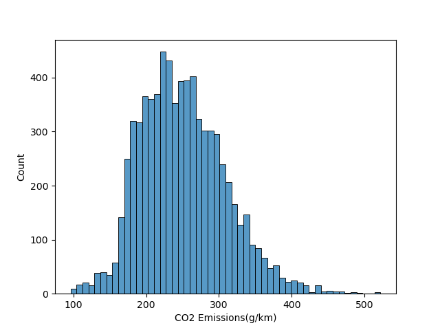
and if we visualize it as a histogram using pandas, we can see that the emissions of co2 are centred around 200 - 270 g/km
let's see how the vehicle class affect the co2 emissions:
co2_data.select('Vehicle Class', 'CO2 Emissions(g/km)').show(5)
+-------------+-------------------+
|Vehicle Class|CO2 Emissions(g/km)|
+-------------+-------------------+
|      COMPACT|                196|
|      COMPACT|                221|
|      COMPACT|                136|
|  SUV - SMALL|                255|
|  SUV - SMALL|                244|
+-------------+-------------------+
only showing top 5 rows
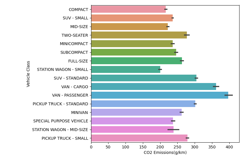
and if we visualize it using a bar chart, we see that cargo vans and passenger vans seems more polluting, while small and compact cars are less polluting:
let's explore how fuel type affect co2 emissions
co2_data.select('Fuel type', 'CO2 Emissions(g/km)').show(5)
+---------+-------------------+
|Fuel type|CO2 Emissions(g/km)|
+---------+-------------------+
|        Z|                196|
|        Z|                221|
|        Z|                136|
|        Z|                255|
|        Z|                244|
+---------+-------------------+
only showing top 5 rows
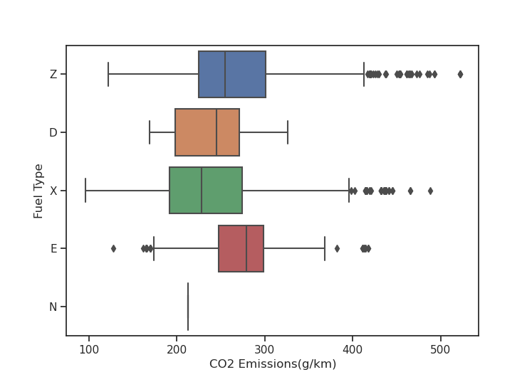
if we visualize that in a bow plot, we can see that cars using fuel type E (Ethanol (E85)) has higher median level of co2 emissions while cars using fuel type X (Regular gasoline) have lower median and so it is less polluting:
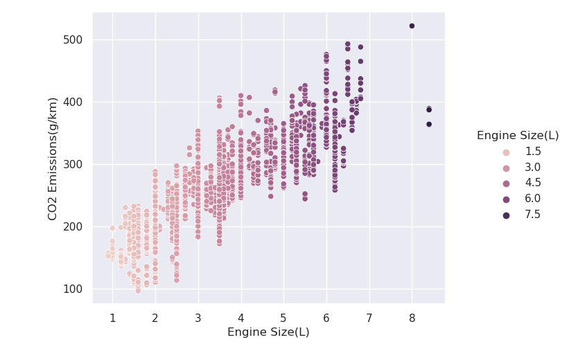
now let's find if the engine size has affect on co2 emissions
co2_data.select('Engine Size(L)', 'CO2 Emissions(g/km)').show(5)
+--------------+-------------------+
|Engine Size(L)|CO2 Emissions(g/km)|
+--------------+-------------------+
|           2.0|                196|
|           2.4|                221|
|           1.5|                136|
|           3.5|                255|
|           3.5|                244|
+--------------+-------------------+
only showing top 5 rows
since we have 2 continuous variables, we can use scatter plot to visualize them:
2 Build Random Forest Regression Model
now after we're done some visual overview of data , let's move to create the random forest model. let's start by import the modules we are going to preprocess our data.
from pyspark.ml.feature import VectorAssembler, StringIndexer, OneHotEncoder
we will do one step at a time for preprocessing data, and store them as stages in our pipeline:
stages = []
we will start with categorical columns
categoricalColumns = ['Make', 'Model', 'Vehicle Class', 'Transmission', 'Fuel Type']
# in the next snippet, and for every column we will label-encode categorical values by labeling and add the suffix 'Index' to those columns, plus we encode them using OneHotEncoder and adding suffix 'Vector' to column names. after that we will add them to stages pipeline:
for col in categoricalColumns:
...     indexer = StringIndexer(inputCol=col, outputCol=col + "Index")
...     encoder = OneHotEncoder(inputCols=[indexer.getOutputCol()],
...     outputCols=[col + "Vector"])
...     stages += [indexer, encoder]
...
after that comes numerical columns:
numerical_columns = ['Engine Size(L)', 'Cylinders', 'Fuel Consumption City (L/100 km)', 'Fuel Consumption Hwy (L/100 km)']
now we assemble the numerical and categorical variables to make them in one Vector assembler column called 'features' , then we append this assembler as another step in our stages:
assembler_inputs = [column + 'Vector' for column in categoricalColumns] + numerical_columns
assembler = VectorAssembler(inputCols=assembler_inputs, outputCol="features")
stages += [assembler]
as we have all our preprocessing stages setup, we can see those stages, where the vectorAssembler at the very end:
stages
[StringIndexer_00a16287889f,
    OneHotEncoder_fcfbea40fb15,
    StringIndexer_27918f0286eb,
    OneHotEncoder_13b5d4a0512f,
    StringIndexer_811b35fa16ce,
    OneHotEncoder_5d178c75064f,
    StringIndexer_9db84853fc4d,
    OneHotEncoder_af8005429dc3,
    StringIndexer_a95bd9ba6c90,
    OneHotEncoder_2d945e708e9c,
        VectorAssembler_0faf10f64957]
now, let's instantiate the machine learning pipeline and pass our stages we created, and fit the co2 emissions data with the pipeline model:
from pyspark.ml import Pipeline

pipeline = Pipeline(stages=stages)
pipeline_model = pipeline.fit(co2_data)
now we have to transform the data with the model , by passing the 'features' column which combine al the interesting columns along with the label column we are looking to predict (CO2 Emissions(g/km)):
co2_data_transformed = pipeline_model.transform(co2_data)
co2_data_transformed.select('features', 'CO2 Emissions(g/km)').show(5,truncate=False)
+------------------------------------------------------------------------------------------+-------------------+
|features                                                                                  |CO2 Emissions(g/km)|
+------------------------------------------------------------------------------------------+-------------------+
|(2142,[30,198,2095,2130,2135,2138,2139,2140,2141],[1.0,1.0,1.0,1.0,1.0,2.0,4.0,9.9,6.7])  |196                |
|(2142,[30,198,2095,2110,2135,2138,2139,2140,2141],[1.0,1.0,1.0,1.0,1.0,2.4,4.0,11.2,7.7]) |221                |
|(2142,[30,1305,2095,2120,2135,2138,2139,2140,2141],[1.0,1.0,1.0,1.0,1.0,1.5,4.0,6.0,5.8]) |136                |
|(2142,[30,1903,2093,2108,2135,2138,2139,2140,2141],[1.0,1.0,1.0,1.0,1.0,3.5,6.0,12.7,9.1])|255                |
|(2142,[30,296,2093,2108,2135,2138,2139,2140,2141],[1.0,1.0,1.0,1.0,1.0,3.5,6.0,12.1,8.7]) |244                |
+------------------------------------------------------------------------------------------+-------------------+
only showing top 5 rows
now let's split the data between training (70 %) and test data (30 %):
co2_data_train, co2_data_test = co2_data_transformed.randomSplit([0.7, 0.3], seed=1)
you can check how many records assigned each:
co2_data_train.count()
5199
co2_data_test.count()
2186
let's instantiate the random forest regressor estimator object.
this is an ensemble learning model that will train a different number of different decision trees and the final output of the model will be an aggregation of the predictions of the individual decision tree models .
a sub-sampling rate of 0.8 means that each tree will be trained on a random 80 % of training data. numTrees of 5 means random forest will include 5 trees(5 individual learners):
from pyspark.ml.regression import RandomForestRegressor

random_forest = RandomForestRegressor(labelCol='CO2 Emissions(g/km)', subsamplingRate=0.8, numTrees=5)
let's train our model by filing it with train data:
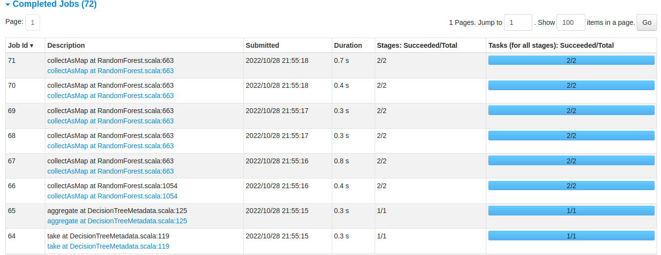
random_forest_model = random_forest.fit(co2_data_train)
and if you look to Spark UI ,you find several jobs' spine up for that process:
Test Random forest model
now after we train our model, we are ready to use it for the predictions.
let's feed and transform the test data into our model:
predictions = random_forest_model.transform(co2_data_test)
predictions.select('prediction', 'CO2 Emissions(g/km)', 'features').show()
+------------------+-------------------+--------------------+
|        prediction|CO2 Emissions(g/km)|            features|
+------------------+-------------------+--------------------+
| 193.1399265652559|                192|(2142,[30,198,209...|
| 193.1399265652559|                199|(2142,[30,198,209...|
| 220.0907558239919|                210|(2142,[30,1353,20...|
| 220.0907558239919|                210|(2142,[30,1354,20...|
| 220.0907558239919|                210|(2142,[30,1354,20...|
| 261.4051122117478|                255|(2142,[30,373,209...|
|250.98018357858123|                252|(2142,[30,373,209...|
|247.52229785463857|                261|(2142,[30,910,210...|
|250.98018357858123|                244|(2142,[30,296,209...|
|250.98018357858123|                244|(2142,[30,296,209...|
|250.98018357858123|                250|(2142,[30,296,209...|
|233.49196915418855|                230|(2142,[30,931,209...|
|202.37901984736186|                177|(2142,[30,730,209...|
|202.37901984736186|                180|(2142,[30,730,209...|
|202.37901984736186|                190|(2142,[30,730,209...|
| 193.1399265652559|                191|(2142,[30,394,209...|
| 193.1399265652559|                205|(2142,[30,394,209...|
|218.75830263602424|                209|(2142,[30,956,209...|
|233.49196915418855|                228|(2142,[30,395,209...|
|227.08160974665074|                225|(2142,[30,960,209...|
+------------------+-------------------+--------------------+
only showing top 20 rows
from a visual view we can see that our model predict pretty well by compare the prediction of co2 emissions with the actual one in 'CO2 Emissions(g/km)' column :

we can confirm that by evaluating the model on test data.
# let's invoke the random forest regressor evaluator by passing the prediction column along with the original column of co2 emissions. then call the evaluate function and use R-squared as a metric:
from pyspark.ml.evaluation import RegressionEvaluator
evaluator = RegressionEvaluator(labelCol='CO2 Emissions(g/km)', predictionCol='prediction')
r2 = evaluator.evaluate(predictions, {evaluator.metricName: 'r2'})
you can see how random forest regression did perform on the test data
print('R² over test data is : ' + str(r2))
R² over test data is : 0.9516606706224755
the R² score is of value 0.95 which means the predictions get correct by 95 % on test data, which is very good score.